This algorithm is designed to provide a tool for quickly modeling large datasets that represent horizontally layered but laterally discontinuous materials or data such as geochemistry or geophysical properties.  Because speed was the primary concern during development, this algorithm does not support the faulting tools built into some of the other RockWorks modeling algorithms.

Layer Height:  For each layer with the output model, this algorithm extracts all of the control points within a horizontal parallelopiped.  The height of this parallelopiped is determined by the Layer Height setting which is a multiple of the Voxel Height (Figure 1).  For example, if the Layer Height is set to 3.0 and the Voxel Height (aka Z-Spacing) is set to 1 meter, the parallelopiped will be 3 meters high.  This means that only the points which are 1.5 meters above or below the midpoint of a model layer will be included in the interpolation.

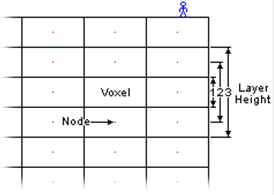
Figure 1

Weighting Exponent:  The voxel values within each layer are estimated based on an inverse-distance weighting algorithm that only uses the control points within the parallelopiped.  In essence, the algorithm creates a block model by stacking gridded models in which the Weighting Exponent determines the influence of the surrounding points on the voxel value estimation (Figure 2).

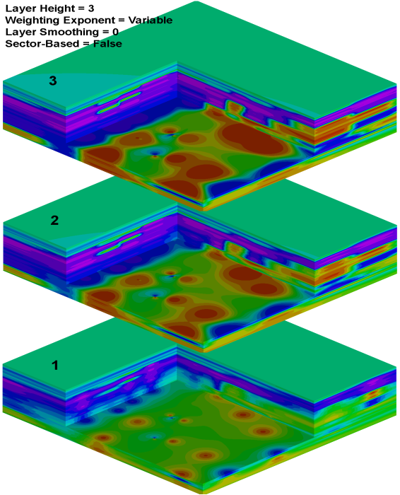
Figure 2

Layer Smoothing:  Unlike the Smoothing option within the Special Options menu, the Layer Smoothing within the IDW Layered sub-menu is optimized (multi-threaded) for this particular algorithm.  Specifically, a 7x7 voxel distance-weighted box filter will be applied to all of the voxels within each parallelopiped followed by a simple averaging of vertically adjacent voxels.  Accordingly, the Special Options / Smoothing option is not shown when the IDW Layered algorithm has been selected.

Sector-Based Searching: If enabled, the IDW Layered algorithm will only use the specified number of closest points within each directional sector relative to the voxel being interpolated.  This can be a useful tool when dealing with clustered or co-linear control points.  Be forewarned, however, that the time required to perform these searches increases with the number of sectors and the number of points used within each of these sectors.

 For example, interpolating a large model (5.8m voxels) based on a large dataset (10,000 points) using four search sectors (90 degree spacing) took approximately 3 minutes compared with the 71 minutes required to interpolate a model that used 72 sectors (5 degree spacing).

No Sector-Based Searching:  Not using Sector-Based Searching is a subjective decision based on personal preferences, the data distribution, and the nature of the geology being modeled.  If the data is evenly distributed (e.g., downhole geochemical data from uniformly spaced wells) modeling without sector-based searching may be preferable.  Not using the sector-based searching is also much faster.

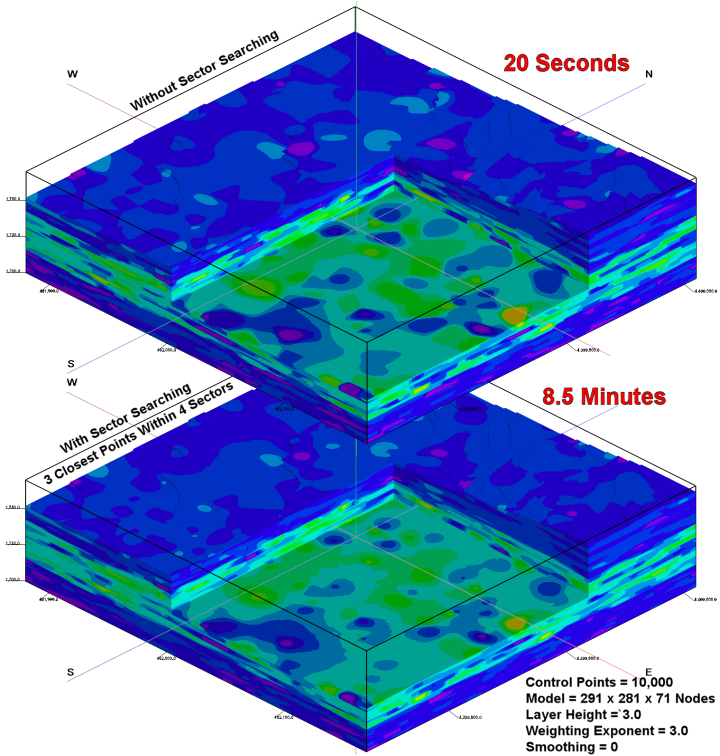
Figure 3

To illustrate how this algorithm works, consider a random dataset with 10,000 XYZG points (Figure 4).  To provide a comparison (Figure 5), creating a 301x301x101 voxel model using the IDW Anisotropic algorithm without any smoothing or other filtering required approximately 15 minutes while the creation of a model using the IDW Layered algorithm configured with a Layer Height equal to the voxel height required approximately 13 seconds.  In addition to the speed difference, note how the minimal Layer Height (1 voxel) has implicitly compressed and laterally connected features.  The degree of compression and connection is controlled by a combination of the Layer Height, the Weighting Exponent, and the Smoothing.  For example, if this data represents volcanic ejecta that has been flattened by compaction (e.g., fiamme), the IDW Layered model is perfect.  Conversely, if the data represents geology that has been churned and de-compacted by a bulldozer, the IDW Anisotropic model is more realistic.

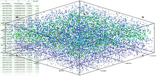
Figure 4

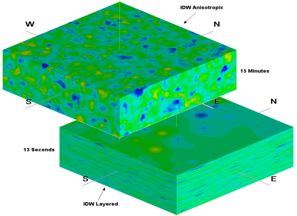
Figure 5

When considered independently, the Layer Height determines the data “connectedness” (Figure 6), however the Layer Smoothing (Figure 7) also determines how isolated features will be consolidated.

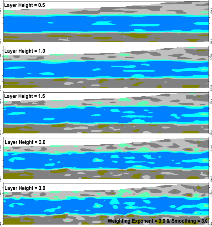
Figure 6

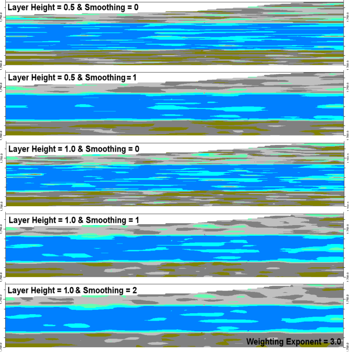
Figure 7

The Weighting Exponent can also be used to influence the lateral variability of the output (Figure 8).  Higher Weighting Exponents increase the lateral heterogeneity while lower Weighting Exponents increase the lateral homogeneity.

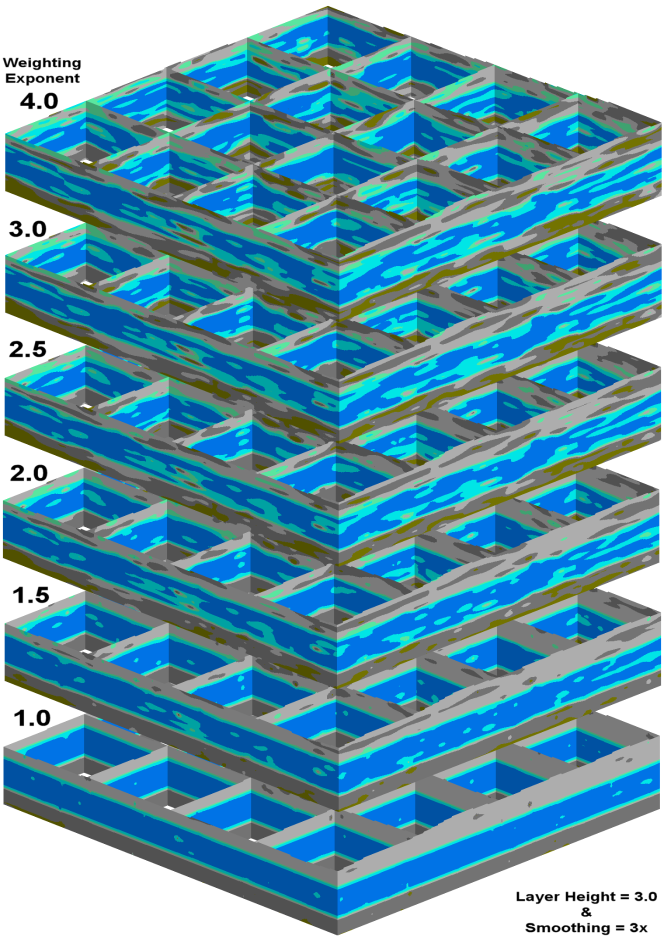
Figure 8

When in doubt, start with the following settings and examine the output (Figure 9):

Layer Height = 2

Weighting Exponent = 2

Layer Smoothing = 1

Sector-Based Searching = Disabled

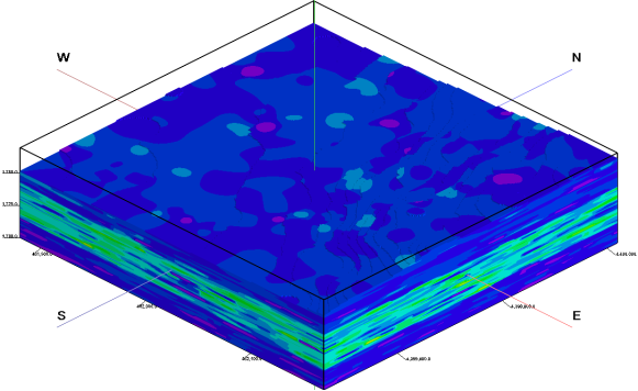
Figure 9

To increase the vertical connections, change the Layer Height from 2 to 3 (Figure 10).

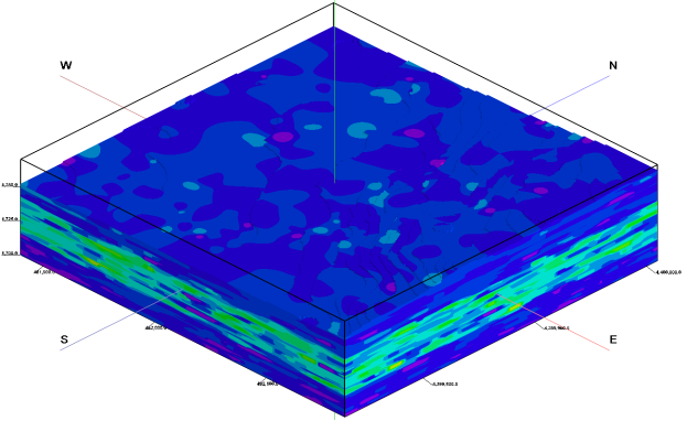
Figure 10